Will player X make it at least 5 years in the league?
Many sports fans find it irresistible to play the role of “armchair general manager” and second-guess any and all personnel decisions of their favorite team. From draft picks to free-agent contracts to trades…every move made will be scrutinized by talking heads, newspaper sports columnists, message boards, etc. It’s not uncommon to conjure up complex trading scenarios that would never happen in real life and curse the front office for not pursuing the “one missing piece” or going “all-in” because this could be OUR YEAR! However, there often isn’t sound analysis behind these opinions. Most casual fans are using the “eye test” and surface-level statistics to decide which young and unproven players they covet.
Once a player truly breaks out and achieves superstar status, he becomes a known quantity to the entire league, and the window of opportunity for acquisition or cost control has passed. What if there was a way to determine whether a player would achieve long-term success simply from his rookie year statistics? My objective was to do just that by building a binary classification model using libraries from sci-kit learn.
The Data: A first look and some feature engineering
The dataset was fairly straightforward:
There are 19 numeric features, player names, and the “target” column which identifies whether or not the player’s career lasted at least 5 years (our given threshold for this classification task).
Before doing anything else, I researched some common advanced NBA metrics and decided to engineer a few additional features to include in the dataset. All of the below features were derived by combining and/or manipulating some of the features that had already been provided.
Feature Engineering:
- True Shooting Percentage: Per Wikipedia, “a statistic that measures a player’s efficiency at shooting the ball”. Intended to be a more comprehensive metric than any of its individual shooting components.
raw_df['TSA'] = raw_df['FGA'] + (0.44*raw_df['FTA']) raw_df['TS%'] = raw_df['PTS']/(2*raw_df['TSA']) - 3NG (3 point net gain) is a metric borrowed from a Towards Data Science blogpost using formula 3NG = 3P Made (3 - EV) - (3P Missed EV)) where EV is expected number of points per possession, for which we can substitute 1.06 for NBA purposes
raw_df['3NG'] = (raw_df['3P Made'] * 1.94) - ((raw_df['3PA'] - raw_df['3P Made'])*1.06) - TOV%: An estimate of turnovers per 100 plays (utilizes part of the TS% equation), from basketball-reference.com
raw_df['TOV%'] = (raw_df['TOV'] * 100)/(raw_df['TSA'] + raw_df['TOV']) - An original metric created to combine counting stats that change the expected flow of the game and yield an “extra” possession
raw_df['Poss_Added'] = raw_df['STL'] + raw_df['BLK'] + raw_df['OREB']
Problems with the Data:
When I first started doing Exploratory Data Analysis, it seemed like I wouldn’t need to do much to clean it up. But the deeper I dug, the more issues I uncovered:
Misclassification
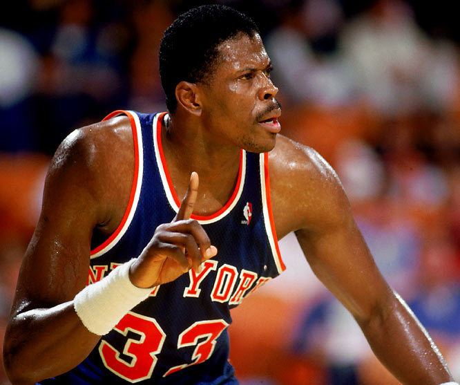
A number of players simply had the wrong value in the target column applied, which made me doubt the accuracy of the ground-truth labels in general. Some prominent examples abound, such as Hall of Famer Patrick Ewing:

Attention dataset curator: You do not want to get on this man’s bad side…
Duplicated Data:
There were a number of players represented twice. Some had identical stat lines but different target values, while others had two rows of stats that clearly seemed to represent two different players.
This line of code returned 59 rows of output:
raw_df[raw_df.duplicated(subset=['Name', 'GP'], keep = False)]
- Those with identical stats comprised a large proportion of the misclassified subset. They simply had two rows, one with target “0” and one with target “1”. It was painful and laborious to research and clean up, but it had to be done to ensure the integrity of the models we would later build.
- For those with different stat lines, I cross-referenced another dataset that was referenced as one of the canonical sources. I got some unexpected practice writing SQL statements to figure out who those stats actually belonged to (generally the first or last name matched the other player whose name was duplicated), then made the necessary changes to my data using pandas.

Here’s Carlos Boozer, originally one of two players listed as Carlos Rogers.
Inclusion of recent draft picks with incomplete statistics
- This was an even bigger challenge. There were a healthy number of players in our dataset who were drafted between 2013-2016. When the dataset was published, 5 years hadn’t yet elapsed counting from their rookie seasons, so it was impossible to classify them as a “1” at the time. However, they were all defaulted to “0”, i.e. it was assumed that none of them would reach the 5 year threshold. To make matters worse, all of the 2016 players had only partial-season statistics (from roughly the first half of their rookie seasons).
- For those players who could now be properly judged (from 2014 and earlier), I reclassified them based on actual career longevity.
- The 2016 player set was too problematic due to the partial-season stats, so I chose to drop that subset of players entirely.
- The 2015 player set was retained as holdout data (but NOT included in our train/test data since all labels defaulted to “0”).
Multicollinearity
I didn’t have any categorical features, so one-hot encoding was unnecessary. I did, however, have quite a bit of multicollinearity to deal with as a lot of my features were derivations of others and naturally correlated (eg. more minutes played leads to higher counting stats such as points and rebounds simply because the player spends more time on the court and has more opportunities to make an impact on the game).

This primarily presented an issue for logistic regression and not tree-based models, so I removed several features to create a separate dataset for the purposes of logistic regression.
Modeling and Evaluation
Comparing out-of-the-box models
After data cleaning, I found that my data contained about 67% “successful” samples. This represents the baseline number upon which we would try to improve. If we created a “dumb” model that predicted every player’s career would last at least 5 years, it would be right about 67% of the time.
I fit several classifiers with default parameters to see how they’d fare initially.
| Model Name | Accuracy Score | F1 Score | Computational Time |
|---|---|---|---|
| Logistic Regression | 0.7342 | 0.8117 | 0.0214 |
| XGBoost | 0.7342 | 0.8082 | 0.1222 |
| Random Forest | 0.7247 | 0.7953 | 0.0280 |
| Gradient Boosting | 0.7215 | 0.8044 | 0.1787 |
| K-Nearest Neighbors | 0.6930 | 0.7749 | 0.0091 |
| AdaBoost | 0.6899 | 0.7752 | 0.2113 |
| Decision Tree | 0.6677 | 0.7518 | 0.0131 |
Surprisingly, Logistic Regression was at the top, but I wasn’t able to improve on it any further. I chose to continue with simple decision trees, random forests, and some boosted ensemble models.
Decision Tree
Predictably, my first decision tree without tuning was incredibly overfitted, with the training set accuracy close to 100% but the testing set underperforming my baseline. This tree was way too deep and creating very granular splits - we ended up with 293 nodes!

After tuning hyperparameters, the trees were much simpler and easier to interpret, but the metrics were about on par with logistic regression.

Random Forest
A collection of trees, each of which uses a subset of features and data for each tree rather than the entire dataset. This should be less susceptible to noise and overfitting…and as expected, the results were better than a single tree once the hyperparameters were tuned.
XGBoost
XGBoost is one of many popular “ensemble” methods which use a weak learner (such as a decision tree) to begin, then iteratively builds stronger and stronger models by focusing on what the weak learner predecessors misclassified and tuning on those areas. Gradient descent is incorporated into this process so that the parameters eventually converge on their optimal values, which generally means that for complex problems, some sort of gradient boosted algorithm will be the best performer. Be forewarned that tuning the hyperparameters can be very computationally expensive though.
Classification Report for XGBoost Testing Set (weighted averages):
| precision | recall | f1-score | support |
|---|---|---|---|
| 0.74 | 0.75 | 0.74 | 316 |
The feature importances with XGBoost can be seen below:

Our final XGBoost model resulted in an accuracy improvement of more than 8% from our baseline. This appears to be our best model in terms of accuracy and F1-score (a balanced score that weights precision and recall equally).
I also tested some unseen data (the 2015 rookies that were removed from the initial dataset) and achieved about an 85% accuracy vs. our own human predictions based on the first four years of their playing careers. Of course this was a small sample size, but a reassuring result nonetheless.
Final thoughts:
Who cares about predicting NBA career length? What’s the business case for something like this?

The truth is that predictive analytics have quickly become a quintessential component of professional sports and the very consequential decision-making (read: handing out multi-million dollar contracts) that occurs at the highest level of each sport. In fact, most front offices now employ at least a handful of full-time data scientists. I have no doubt that models considerably more complex than this are utilized on a regular basis to facilitate internal personnel evaluation in professional leagues. Player agents can also leverage data to advise their clients on which areas to dedicate their focus and training, or to pitch their clients to teams when free agency looms.
While this dataset used rookie-year statistics, the same processes can be applied to high school and college statistics to create projections and prepare for annual amateur drafts. Clubs who routinely succeed with those draft picks end up with cost-controlled assets who will easily outperform their salaries and they’ll have much more flexibility to build out their rosters via free agency, trades, etc. So while this may seem like a trivial exercise at first glance, professional sports organizations consider this kind of analysis very seriously…and for good reason.